TOF Sequential Single Peak Fits and loading curve
Introduction: A common analysis of diffraction data obtained from a polycrystalline sample subjected to a changing uniaxial load is to follow the behavior of fitted single peaks. The data sets considered here were obtained on the Vulcan diffractometer at SNS, Oak Ridge National Laboratory. The layout of the instrument

has panels of detectors on both sides of the sample (in this case a ¼” stainless steel rod) oriented so that the loading axis is 45° to the incident neutron beam. Thus one detector “Bank 1” only views crystallites with diffraction vectors parallel to the loading direction while the other “Bank 2” only views crystallites with diffraction vectors perpendicular to the load. In such an experiment, as the load is increased (as a tension) we would expect that the reflections would shift to higher d-spacings in Bank 1 and those seen in Bank 2 would shift to smaller d-spacings. If the load is a compression, then the responses in the reflection positions would be reversed. The shift records the response “strain” of the crystal lattice to the load “stress”. The particular experiment done here was to subject the steel rod to ten tension/compression cycles over 13 hours recording a diffraction pattern from the two detectors each minute yielding ~800 data sets. The 1st loading cycle was done slowly over ~4.5hrs and the remaining ones done ~1hr each; we will focus on just the 1st cycle for this tutorial comprising 61 powder patterns. Note that menu entries and user input are shown in bold face below as Help/About GSAS-II, which lists first the name of the menu (here Help) and second the name of the entry in the menu (here About GSAS-II).
If you have not done so already, start GSAS-II.
Step 1. Import the powder data for sequential fitting
Use the Import/Powder data/from GSAS powder data file menu item to read the data file into the current GSAS-II project.
A file selection dialog will be shown; its appearance will depend on your OS. Change the search directory to TOF Sequential Single Peak Fit/data and then select all the *.gsa files (435.gda-495.gda) and press Open. A small popup window will appear
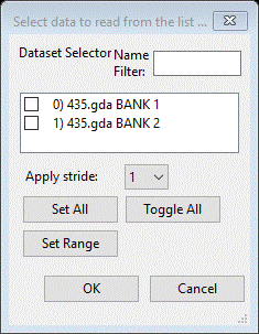
Select just 435.gda BANK 1 and press OK. After a pause while the data is read the main window will highlight the last entry (PWDR 495.gda Bank1)
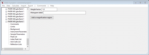
and show the powder pattern
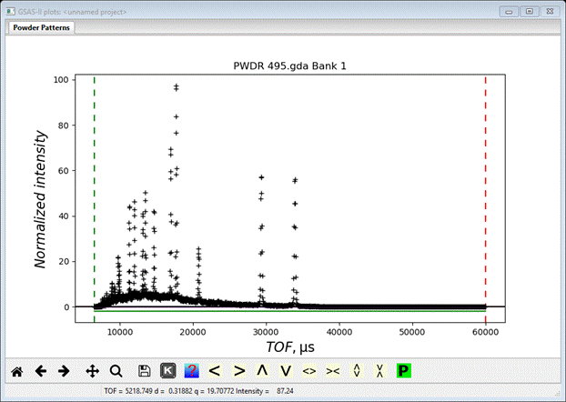
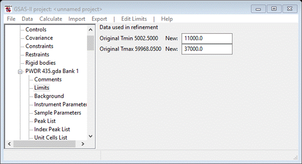
You may start here but it is slightly better to start with the 1st data set; select PWDR 435.gda BANK 1 from the tree (press the ‘+’ to expand it) and select Limits

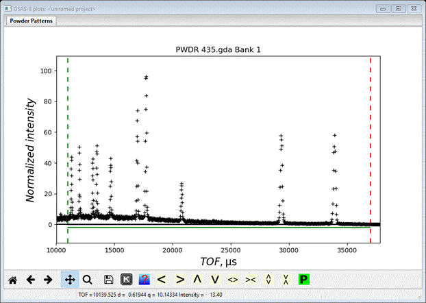
The plot shows the current limits as vertical green & red dashed lines.
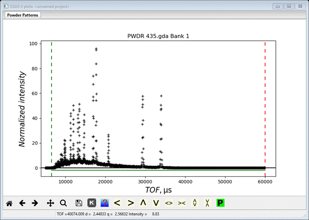
Set the Tmax value to 37000 and the Tmin to 11000; this will encompass the 1st 10 peaks of the powder pattern.
Next copy these limits to the other PWDR data sets; do Edit Limits/Copy. A selection dialog box will appear
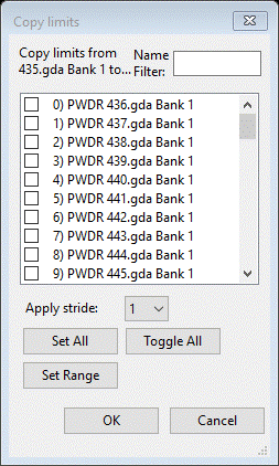
Do Set All and press OK; the limits will be copied to the other histograms.
Step 2. Peak fitting for 1st data set.
In this step we will select the 10 reflections for single peak fits and fit them. Select Peak List for the 1st PWDR data set; it will be empty. To populate it do Peak Fitting/Auto Search; this will find the 10 peaks and put them in the list and mark them on the plot with vertical blue lines.
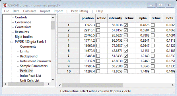
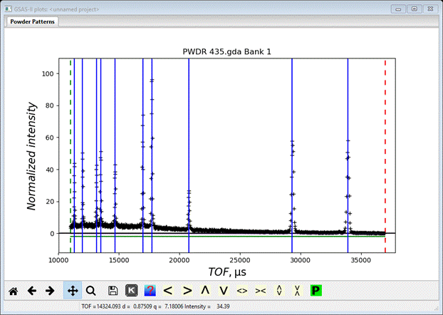
Next do Peak Fitting/Peakfit from the menu; a file dialog will appear asking for a file name (I used “steel”) to create a new project. The refinement will then do the initial fit to the 10 peaks varying only intensity and background (default of 3 term Chebyschev polynominal). The result is
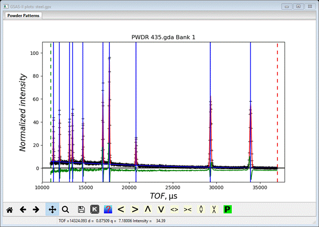
and shows the need for further refinement for both position & peak width. To do this double click on the refine column heading for position and sigma selecting ‘Y’ from the popup in each case. When done the Peak List should look like

with check marks in three columns. Then do Peak Fitting/Peakfit; the fit will be much improved
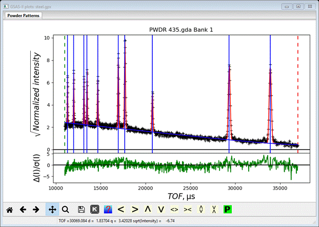
I’ve pressed both ‘W’ to get the DI/s(I) curve and ‘S’ to see sqrt(intensity) on the plot. The residual for the fit (see console for this) is ~14%; it perhaps could be improved by more background terms but this will not have much effect on the peak parameters.
Step 3. Sequential peak fit
To prepare for the sequential peak fitting we need to copy the results from fitting 10 peaks to the other PWDR histograms. Do Peak Fitting/Peak copy; a selection dialog will appear. Do Set All and press OK; the peak fit data will be copied to the other PWDR histograms. Next do Peak Fitting/Seq Peakfit; again a selection dialog will appear

Notice this one does offer the possibility of doing the fit in reverse (i.e. start from the last PWDR entry) and also to copy the result from one fit to the next one in sequence as possibly better starting values for its refinement. We’ll not bother with either here. Do Set All and press OK; GSAS-II will rapidly do the 10 peak fitting on all 61 PWDR histograms. The final sequential result is displayed
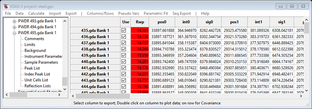
The table is quite large with >30 columns and 61 rows so I’ve shown only a bit of it. If you select a row, the plot will show the corresponding PWDR plot and fit; this is the same as selecting a PWDR entry in the main data tree (this will respond to arrow keys to step from one PWDR entry to the next and show the corresponding plot). For your first view of the sequential result double click on the pos0 column heading; the variation in this value across the sequence will be plotted; each point has the error bar obtained in the refinement
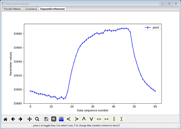
This shows the result of a loading/unloading cycle essentially in time (data collection sequence number). More interesting would be to show the dependence on load; we need to set the applied load used for each data set.
Step 4. Import applied load table
A hard way to enter the loads is to do each one by hand; they are entered in the Sample Parameters tree item for each PWDR entry. Select that now for the 1st PWDR entry
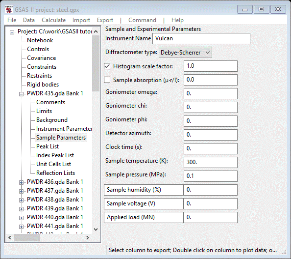
Notice there is an entry at the bottom of the table for Applied load (MN); you’d have to fill that in for every PWDR data set. However, there is an easier way since a metadata file with this information was provided by the Vulcan Instrument Scientist. To access it do Command/Load all; a file selection dialog will appear. Choose 28902sampleenv_chopped_mean.txt and open it; a Select columns dialog box will appear

Looking over the column headings, one is marked “stress” and another is marked “force”. Their ratio is presumably the cross-section area of the steel rod (in mm2). So (counting from zero) the column we want for Applied load is Column #6 (1st value ~169.45); select Applied load from the pulldown under the heading. The table should show
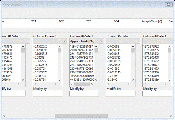
Notice you can apply conversion factors to the column of values if desired; just enter it in the Modify by box.
Press OK; all the Sample Parameters tables will be updated filling in the appropriate values for Applied load.
Select Sequential peak fit results from the data tree

Applied load is a new column entry in the table; double click the pos0 column heading. A new plot will appear

which is unchanged from before. Place the cursor anywhere on the plot (i.e. select it) and press the ‘s’ key; a popup dialog will appear.

Select Applied load and press OK. The plot will change (you may have to select ‘pos0’ again)
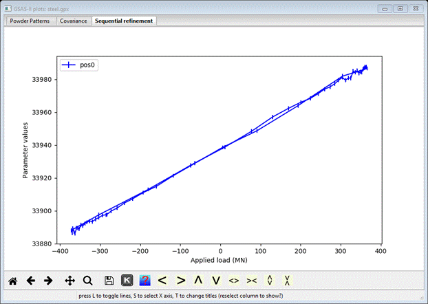
This shows the perfectly linear response of peak position with applied load. Select another pos parameter; the plot will change

Pos1 shows hysteresis in a load/unload cycle; some of other peaks will be similar while others will resemble pos0. This would be a good place to do File/Save project.
Step 5. Sequential data fitting
Since pos0 gives a nice straight line response to load, we can try to extract the Hookes Law elastic coefficient for that reflection. To do this we must find the strain from the peak position shift from the zero load value. First select pos0 from the Sequential results table.

Using the cursor, find the zero load point on the curve and note value for pos0; it will show up in a tool tip displayed as the cursor is positioned. I found pos0=33937 at load=0. We will use this to compute the strain0 = (pos0-33937)/33937; we want this as a new column in the table. To do this do Pseudo Vars/Add Formula; a new window “Expression Editor” will appear

Enter (x-33937)/33937 in the box after the + sign; the window will be redrawn

Select ‘Global’ from the pulldown next to the ‘x’ (your variable name in the equation); a new selection box will appear. Choose pos0 (pos for the filter can help reduce the choices) from the list and press OK. The window is again redrawn
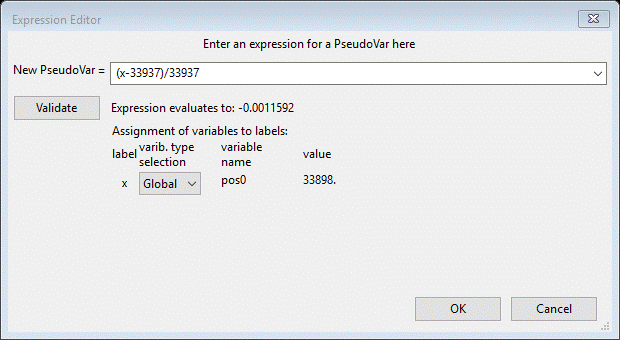
All looks properly filled in so press OK; the sequential table will now have a new column at the end with the entered equation as its name

Click on that column heading to see its plot vs load
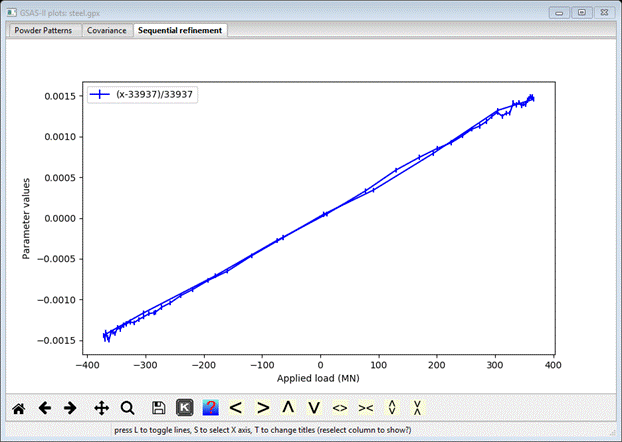
This is what we want to fit to get the Hookes Law coefficient. Do Parametric Fit/Add equation; the Expression Editor window will appear

Select Global from the pull down on the left of the = sign and pick (x-33937)/33937 from the list. Then enter m*y+b in the box to the right of the = sign. NB: x was used earlier so we can’t use it here. That establishes the equation you are trying to fit to the data. The window will change to give
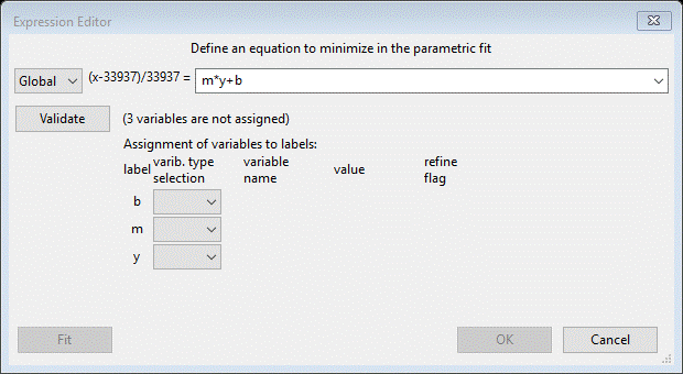
For the three pull downs, b is Free, m is also Free (the fitting variables) and y is a Global; select Applied load for it. The Editor will change again

Press Fit or even just OK. The console will show the fitting result
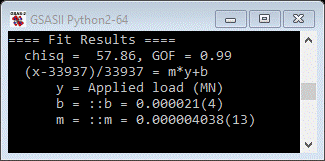
And the plot will show the best fit line in red; it nicely matches the data.

The resulting Hookes Law coefficient is 40.38(13)x10-6 MN-1 for this reflection (austenite 111). This end the tutorial; save the project if desired. You can further explore the sequential results and perhaps extract Hookes Law coefficients for the other reflections that show no hysteresis. If you want the look at Bank 2 data (the opposite detector) you should start with a fresh GSAS-II project file and follow this tutorial for it. The ratio of the corresponding slope for the austenite 111 reflection with what we found here should be the Poisson ratio.